Overview

It aims to control a position and/or rotation of a part of the robot in natural 3D space. There are different mathematical ways to represent the position and the orientation of a rigid body in space. ALMath offers two ways to represent a solid in 3D:

Transform: it is one of the best way to describe a solid in space. It is composed of a rotation matrix and a translation.
Position6D: it is a compact representation. In basic case, it could be practical. But this representation has the drawback to have gimbal lock, which is a lost of degree of freedom.

At the end of this section, we describe how to compute the transform from a position6D.

Rotation matrix In our case, a rotation matrix is a 3*3 matrix. In linear algebra, a rotation matrix is a matrix that applies a rotation in Euclidean space.

$R = \left[\begin{array}{ccc} r_1c_1 & r_1c_2 & r_1c_3 \\ r_2c_1 & r_2c_2 & r_2c_3 \\ r_3c_1 & r_3c_2 & r_3c_3 \\ \end{array}\right]$ with $\left\{\begin{array}{c} R^t = R^{-1} \\ det(R) = 1 \end{array}\right.$

The following three basic rotation matrices rotate vectors around x, y or z axis, in three dimensions.

$R_x(\theta) = \left[\begin{array}{ccc} 1 & 0 & 0 \\ 0 & cos(\theta) & -sin(\theta) \\ 0 & sin(\theta) & cos(\theta) \\ \end{array}\right]$

$R_y(\theta) = \left[\begin{array}{ccc} cos(\theta) & 0 & sin(\theta) \\ 0 & 1 & 0 \\ -sin(\theta) & 0 & cos(\theta) \\ \end{array}\right]$

$R_z(\theta) = \left[\begin{array}{ccc} cos(\theta) & -sin(\theta) & 0 \\ sin(\theta) & cos(\theta) & 0 \\ 0 & 0 & 1 \end{array}\right]$

Transform: Homogeneous representation

The homogenous representation is a 4*4 matrix which is composed of rotation and translation part. It represent a solid in 3D.

$H = \left[\begin{array}{cc} R & r \\ 0_{1,3} & 1 \end{array}\right]$

with:

R: rotation part
r = $\left[r_x r_y r_z\right]^t$ : translation part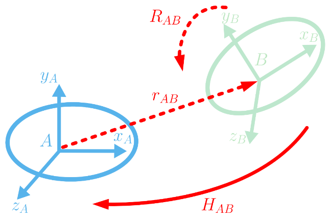

Change Reference

$H_{ab} = \left[\begin{array}{cc} R_{ab} & r_{ab} \\ 0_{1,3} & 1 \end{array}\right]$

$H_{ba} = H_{ab}^{-1} = \left[\begin{array}{cc} R_{ab}^t & -R_{ab}^t r_{ab} \\ 0_{1,3} & 1 \end{array}\right]$

Position6D

A Position6D is a vector of 6 dimensions composed of 3 translations (in meters) and 3 rotation (in radians). The angle convention of Position6D is $Rot_z(w_z) . Rot_y(w_y) . Rot_x(w_x)$ .

$Position6D = \left[\begin{array}{c} x \\ y \\ z \\ z \\ w_x \\ w_y \\ w_z \end{array}\right]$

with:

: translation part (3 scalars)
: rotation part (3 scalars)

Position6D versus Transform

The following equation shows how to compute a transform from a position6D.

$Position6D = \left[\begin{array}{c} x \\ y \\ z \\ w_x \\ w_y \\ w_z \end{array}\right]$ => $H = \left[\begin{array}{cc} R & r \\ 0_{1,3} & 1 \end{array}\right]$ with $\left\{\begin{array}{l} R = R_z(w_z) R_y(w_y) R_x(w_x) \\ r = \left[\begin{array}{ccc}x & y & z \end{array}\right]^t \end{array}\right.$

Basic Example: represente a solid which position is x=1.0, y=-0.5, z=0.4 ad his orientation is 10 degree around x axis. 10 degree is equal to 0.1745 radian. In this basic case, it is very simple to use Position6D.

$Position6D = \left[\begin{array}{c} +1.0 \\ -0.5 \\ -0.4 \\ 0.1745 \\ 0.0 \\ 0.0 \end{array}\right]$ <=> $Transform = \left[\begin{array}{cccc} 1 & 0 & 0 & +1.0 \\ 0 & 0.9848 & -0.1736 & -0.5 \\ 0 & 0.1736 & 0.9848 & +0.4 \\ 0 & 0 & 0 & 1 \end{array}\right]$